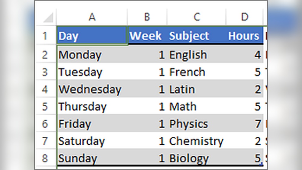
Are you tired of staring at endless rows of numbers and data in Excel that all look the same? Coloring every other row can make your spreadsheet easier to read, help you spot trends faster, and give your work a professional touch.
But if you’re not sure how to do this quickly and efficiently, don’t worry—you’re in the right place. In this guide, you’ll learn simple, step-by-step methods to color every other row in Excel, whether you want to use built-in features or customize your own patterns.
By the end, your spreadsheets will not only look cleaner but will also save you time and reduce errors. Ready to transform your Excel sheets? Let’s dive in!
Select Data Range
Selecting the correct data range is the first step to color every other row in Excel. This action defines which cells will receive the color formatting. It ensures your changes apply only where you want. Proper selection prevents errors and saves time.
Start by deciding the area of your spreadsheet to format. It can be a few rows or an entire table. Click on the first cell in your desired range. Hold and drag the cursor to cover all cells you want to color. Release the mouse button to complete the selection.
You can also select a whole column or row by clicking the column letter or row number. For large datasets, use the keyboard shortcuts. Press Ctrl + Shift + Right Arrow to select cells horizontally. Use Ctrl + Shift + Down Arrow to select cells vertically. These shortcuts speed up the process.
Selecting Cells With The Mouse
Click the top-left cell of your range.
Hold the left mouse button and drag to the bottom-right cell.
Release the button to highlight the area.
Selecting Entire Rows Or Columns
Click the row number to select a full row.
Click the column letter to select a full column.
Use Shift + click to select multiple rows or columns.
Selecting Large Data Ranges With Keyboard
Click the starting cell.
Press and hold Ctrl + Shift.
Press arrow keys to extend the selection.
Use Format As Table
Using the Format as Table feature in Excel is a quick way to color every other row. It automatically applies alternating row colors to your data. This makes your spreadsheet easier to read and more organized.
This method works well for tables that need clear visual separation between rows. Excel offers many built-in styles you can choose from. You can also customize the colors to fit your needs.
How To Select Your Data
Start by selecting the cells you want to format. Click and drag over the range or press Ctrl + A to select all cells in the sheet. Make sure to include all rows and columns you want in your table.
Applying Format As Table
Go to the Home tab on the Excel ribbon. Click the Format as Table button. A menu with different table styles will appear. Choose a style that uses alternating row colors.
Confirm Table Range
A dialog box will pop up asking to confirm your data range. Check that the range matches your selection. If your data has headers, ensure the “My table has headers” box is checked. Click OK to apply the table format.
Customize Table Styles
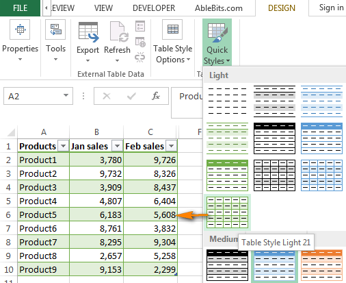
After applying the table, you can change its style anytime. Click the Table Design tab that appears on the ribbon. Select a different style from the gallery for new colors. You can also create your own custom style here.
Benefits Of Using Format As Table
Excel keeps the alternating colors even when you add or delete rows. It also makes sorting and filtering data easier. This method saves time compared to manual coloring or conditional formatting.
Apply Conditional Formatting
Applying conditional formatting in Excel lets you color every other row quickly. This method helps improve data readability and makes your spreadsheet look neat. It uses a simple formula to highlight alternate rows automatically.
Conditional formatting works by checking each row number. It colors rows based on whether the row number is even or odd. This saves time compared to manually coloring rows one by one.
Open Conditional Formatting Menu
Select the cells or the entire table you want to format. Then, go to the Home tab on the Excel ribbon. Click on the Conditional Formatting button. Choose New Rule from the dropdown menu.
Set Up A Formula Rule
In the New Formatting Rule window, select Use a formula to determine which cells to format. Enter the formula =ISEVEN(ROW()) to color even rows. Use =ISODD(ROW()) to color odd rows instead.
Choose A Color Format
Click on the Format button to open the formatting options. Pick a fill color you want for the highlighted rows. Click OK to confirm the color choice. Then, click OK again to apply the rule.
Review And Edit The Formatting
Check your spreadsheet to see the colored rows. To change the color or formula, open Conditional Formatting and select Manage Rules. Edit the rule and save your changes. This keeps your data visually clear and easy to read.
Enter Custom Formula
Entering a custom formula is the key step to color every other row in Excel. This method uses conditional formatting to apply color based on a formula. The formula checks the row number and colors rows accordingly.
Using a custom formula lets you control exactly which rows get colored. It is more flexible than preset options. You can choose to color odd or even rows by changing the formula.
Open Conditional Formatting Menu
First, select the range of cells you want to format. Next, go to the “Home” tab on the Excel ribbon. Click on “Conditional Formatting” in the Styles group. Then, choose “New Rule” from the dropdown menu.
Select Use A Formula To Determine Which Cells To Format
In the New Formatting Rule window, select the option “Use a formula to determine which cells to format.” This option allows you to enter your own formula for formatting. It gives you full control over which rows get colored.
Enter The Formula For Every Other Row
Type the formula =ISEVEN(ROW()) to color even rows. To color odd rows instead, use =ISODD(ROW()). These formulas check the row number and return TRUE for even or odd rows. Excel then applies the format to those rows only.
Set The Format And Apply
Click the “Format” button to choose your fill color. Pick a light color for easy reading. After selecting the color, click “OK” to close the Format Cells window. Finally, click “OK” again to apply the rule to your selected range.
Choose Color Style
Select your data range first to apply color styles. Use Excel’s “Format as Table” or conditional formatting to shade every other row. This improves readability and makes data easier to follow.
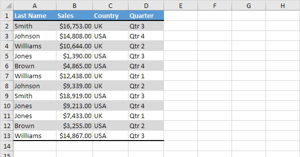
Choosing the right color style makes your Excel sheet easier to read. It helps separate rows visually, reducing eye strain. You can pick colors that match your document’s theme or make data stand out.
Excel offers preset color styles and custom options. Presets are quick and work well for most needs. Custom colors let you personalize your sheet fully. Use soft colors for a clean look or bold colors for emphasis.
Using Preset Color Styles
Excel’s built-in styles save time. They apply color bands automatically across your rows. To find these, select your table and go to the “Format as Table” option. Pick a style that fits your data and preference.
These styles adjust to your table size. They keep alternate rows distinct without extra work. Presets often include light and dark shades for easy reading.
Creating Custom Color Styles
Custom colors allow more control over your design. Use the “Conditional Formatting” feature to add your chosen colors. This method uses formulas to color every other row.
Pick colors that suit your purpose and audience. Soft pastels work well for reports. Bright colors can highlight important data. Make sure the colors contrast enough for clarity.
Tips For Choosing Effective Colors
Choose colors that do not distract from your data. Avoid very bright or clashing colors. Keep it simple with two or three colors at most. Test your color choice on different screens.
Consider color blindness accessibility. Use patterns or borders if needed. Good color style improves readability and makes your sheet look professional.
Credit: www.excel-easy.com
Adjust Formatting Rules
Adjusting formatting rules in Excel helps customize how every other row appears. This step ensures your worksheet looks clear and organized. It also improves readability, making data easier to follow.
You can change colors, set specific rows, or modify the formula to fit your needs. Excel’s Conditional Formatting allows precise control over the look of your rows. Let’s explore how to adjust these rules effectively.
Open Conditional Formatting Rules Manager
Start by selecting the range of cells you want to format. Then, go to the Home tab on the ribbon. Click on Conditional Formatting and choose “Manage Rules” from the dropdown menu. This opens the Rules Manager window.
Here, you see all the existing formatting rules for your selection. You can edit, delete, or add new rules to adjust row colors.
Edit The Existing Formatting Rule
In the Rules Manager, select the rule that colors every other row. Click “Edit Rule” to open the editing window. You will see the formula controlling the formatting, such as =ISEVEN(ROW()) or =ISODD(ROW()).
Change the formula if you want to switch from coloring even rows to odd rows or vice versa. You can also modify the fill color by clicking the Format button. Choose a new color that fits your design.
Create A New Custom Rule
If you want a different pattern or color, create a new rule. Click “New Rule” in the Rules Manager. Select “Use a formula to determine which cells to format.” Enter your custom formula, for example, =MOD(ROW(),4)<2 to color two rows, skip two rows.
Click Format to pick the fill color. Press OK to save the rule. Your worksheet will update with the new alternating pattern.
Handle Hidden Rows
Handling hidden rows in Excel is important when coloring every other row. Hidden rows can disrupt your pattern. If you color rows without considering hidden ones, the colors may look uneven or wrong.
To keep your alternating colors correct, you need to exclude hidden rows from the color pattern. This ensures visible rows follow the correct sequence.
Use A Helper Column To Identify Visible Rows
Create a helper column next to your data. Use the formula
Drag the formula down for all rows. This helps you identify visible rows clearly.
Apply Conditional Formatting Based On Visible Rows
Use conditional formatting with a formula that counts only visible rows. For example, use:
This formula colors every other visible row using the helper column results.
Adjust The Range To Include Only Your Data
Select the exact range of your data without extra rows. This avoids coloring empty rows or outside your data area. Keep your formatting neat and precise.
Test Your Formatting After Hiding Rows
Hide some rows and check the colors. The alternating pattern should stay consistent. This confirms the method works well even with hidden rows.
Remove Alternate Coloring
Removing alternate coloring in Excel helps clear formatting for a fresh look. It simplifies the sheet by deleting row colors quickly. This is useful when you want to reset or change the color style.
You can remove alternate coloring from a whole table or selected rows. Excel offers easy ways to erase colors without disturbing your data. Follow simple steps to clean up your worksheet.
Remove Alternate Coloring Using Clear Formats
Select the rows or range with the colored rows. Go to the Home tab on the ribbon. Click on the Clear button in the Editing group. Choose Clear Formats from the dropdown menu. This removes all formatting, including alternate row colors.
Remove Conditional Formatting To Clear Alternate Colors
Alternate row colors often come from conditional formatting rules. Select the colored cells or entire sheet. Open the Home tab and click Conditional Formatting. Choose Clear Rules, then select Clear Rules from Selected Cells or Entire Sheet. This deletes any rules that apply alternate colors.
Remove Table Style To Delete Alternate Row Colors
If your data is in an Excel Table, it may use a built-in style with alternate row shading. Click anywhere inside the table. Go to the Table Design tab on the ribbon. In the Table Styles group, select None or a plain style. This removes the banded rows color.
Use Keyboard Shortcuts
Using keyboard shortcuts in Excel speeds up your work. It helps you color every other row quickly without using the mouse. This method is simple and efficient for users who prefer using the keyboard.
Keyboard shortcuts save time and reduce repetitive clicking. They make your Excel tasks smoother and more enjoyable. Follow the steps below to apply alternating row colors with just a few keys.
Selecting The Data Range
First, select the cells you want to color. Use Shift + Arrow keys to highlight the range. This method is faster than dragging with the mouse. You can also press Ctrl + A to select the entire sheet if needed.
Opening The Fill Color Menu
Press Alt + H to open the Home tab. Then press H again to open the Fill Color menu. This shortcut lets you pick the color to fill your selected cells.
Applying Color To Every Other Row
After opening the Fill Color menu, use the arrow keys to choose your color. Press Enter to apply it. Then, move down two rows using the arrow keys and repeat. This process colors every other row manually but quickly with the keyboard.
Using Conditional Formatting With Keyboard Shortcuts
Press Alt + O + D to open Conditional Formatting Rules Manager. Then press Alt + N to add a new rule. Use the formula =ISEVEN(ROW()) or =ISODD(ROW()) to color alternate rows automatically.
Set the format by pressing Alt + F to open the Format Cells window. Choose Fill, select a color, and confirm by pressing Enter. This method colors alternate rows dynamically based on your formula.

Credit: www.youtube.com
Credit: www.ablebits.com
Frequently Asked Questions
How Do I Color Every Other Row In Sheets?
Select your data range, go to Format > Alternating colors, and pick a style. Or use Conditional formatting with the formula =ISEVEN(ROW()) to color every other row.
How Do I Mark Every Other Row In Excel?
Select your data range, go to Home > Conditional Formatting > New Rule. Choose “Use a formula” and enter =ISEVEN(ROW()). Pick a fill color and click OK to mark every other row in Excel.
How Do I Highlight Every Other Row In Numbers?
Select your data range in Numbers. Open the Format sidebar, click “Cell,” then choose “Alternating Row Color. ” Pick a style or customize colors to highlight every other row easily.
How Do I Highlight Every 3rd Row In Excel?
Select your rows, go to Home > Conditional Formatting > New Rule. Choose “Use a formula,” enter =MOD(ROW(),3)=0, pick a color, and click OK.
How Do I Color Every Other Row In Excel Quickly?
Use Excel’s “Format as Table” feature to apply built-in alternating row colors instantly.
Can I Use Conditional Formatting To Color Alternate Rows?
Yes, apply a formula like =MOD(ROW(),2)=0 in conditional formatting to color every other row.
What Is The Easiest Way To Highlight Alternate Rows?
Using “Format as Table” is the simplest method to highlight alternate rows automatically.
How To Remove Alternate Row Colors In Excel?
Select the table or range, then clear the formatting or convert the table back to a range.
Can I Customize Colors For Alternate Rows In Excel?
Yes, you can pick custom colors when using conditional formatting or table styles.
Does Excel Support Automatic Row Striping?
Yes, Excel tables automatically stripe rows for better readability.
Conclusion
Coloring every other row in Excel improves data readability. It helps you quickly find and compare information. Using built-in features, you can apply colors easily and save time. Try the alternating colors or conditional formatting methods. Both options work well for different needs.
Keep practicing to make your spreadsheets look clean and organized. This simple formatting trick makes your data clearer and easier to use. Give it a try in your next Excel project.