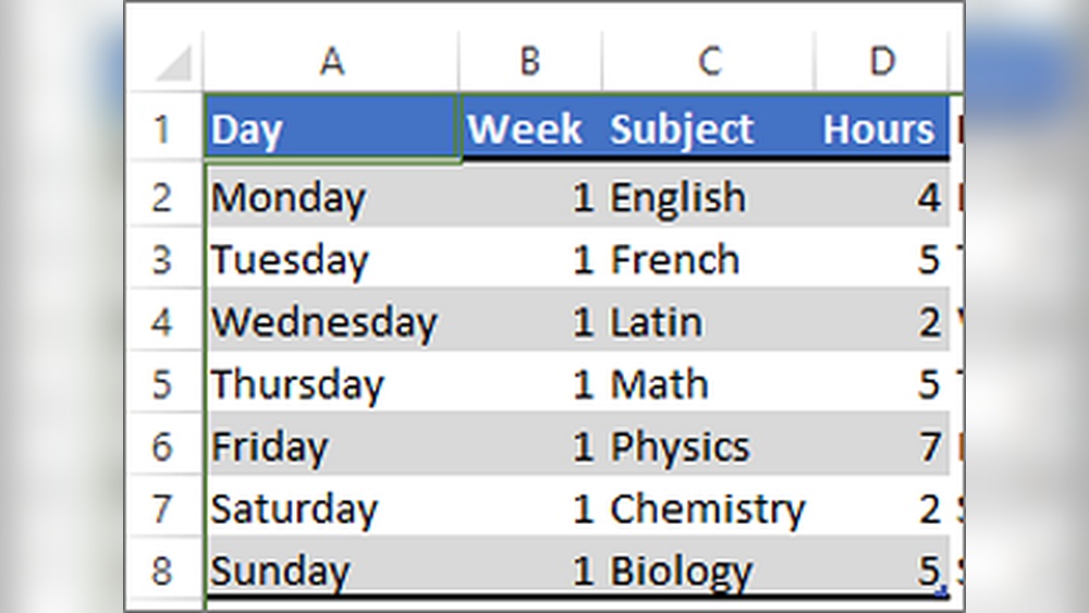
Do you often find yourself scrolling through endless rows of data in Excel and struggling to keep track of your place? Alternating row colors is a simple trick that can make your spreadsheets much easier to read and navigate.
Whether you’re working on a budget, a project plan, or a data report, adding a splash of color to every other row instantly boosts clarity and reduces mistakes. In this guide, you’ll discover easy, step-by-step methods to alternate row colors in Excel—no advanced skills required.
Ready to transform your spreadsheets into neat, eye-friendly tables? Let’s dive in and make your data pop!
Quick Table Formatting
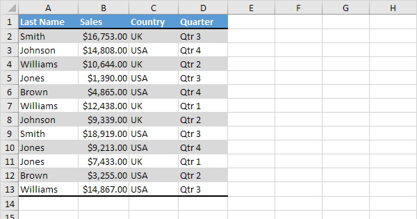
Quick table formatting in Excel helps you add alternating row colors fast. This feature improves readability and makes data easier to scan.
Excel offers built-in styles that apply shading automatically. You do not need complex steps or extra tools.
Using The Format As Table Feature
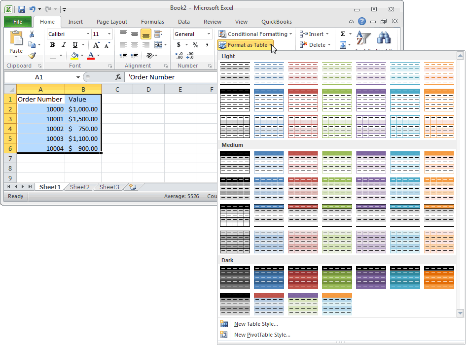
Select the range of cells you want to format first. Then, click the Home tab on the ribbon.
Find and click Format as Table. Choose a style with alternating row colors.
If your data includes headers, check the box that says “My table has headers.” Click OK. Excel applies the colors instantly.
Applying Conditional Formatting For Custom Colors
Select the cells you want to color next. Go to the Home tab again and click Conditional Formatting.
Choose New Rule and then select “Use a formula to determine which cells to format.”
Enter the formula =MOD(ROW(),2)=0 to shade every other row. Click Format, pick a fill color, and press OK twice.
This method lets you pick any color. It works well if you want to avoid full table formatting.
Using Conditional Formatting
Using Conditional Formatting in Excel lets you color rows with precision. It helps highlight every other row automatically. This technique improves readability in large data sets.
This method works well if you want to customize colors beyond the default table styles. It also keeps your data looking clean and professional. The process uses simple formulas and built-in Excel tools.
How To Select The Range For Formatting
First, highlight the cells where you want alternating colors. Make sure to include all rows and columns you wish to format. Avoid selecting extra blank cells to keep the formatting neat.
Creating The Conditional Formatting Rule
Go to the Home tab on Excel’s ribbon. Click on Conditional Formatting, then choose New Rule. Select Use a formula to determine which cells to format. This option lets you apply your own formula for row coloring.
Writing The Formula For Alternating Rows
Enter this formula:
Choosing The Fill Color
Click the Format button after entering the formula. Go to the Fill tab and pick a background color. Choose a light shade for easy reading. Click OK to confirm your choice.
Applying And Managing The Rule
Press OK again to apply the rule to your selected cells. Excel instantly colors the rows based on your formula. You can edit or delete this rule anytime from the Conditional Formatting menu.
Customizing Color Choices
Customizing color choices in Excel makes your spreadsheet clearer and more appealing. Changing the default colors helps highlight data and improve readability. Simple tweaks can match your brand colors or personal style. This section explains how to pick and apply custom colors for alternating rows.
Choosing Colors That Enhance Readability
Select colors with enough contrast for easy reading. Light shades work well for backgrounds, paired with dark text. Avoid very bright or neon colors as they strain the eyes. Soft blues, grays, or pastels usually look neat and professional.
Using The Format As Table Color Picker
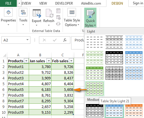
Excel’s Format as Table feature offers preset color styles. You can customize these by selecting a style close to your preference. After applying, use the Table Design tab to pick different colors for header and rows. This method is fast and user-friendly for beginners.
Applying Custom Colors With Conditional Formatting
Conditional Formatting allows precise control over colors. Use a formula to target alternate rows and set any fill color you want. Open the Fill tab and pick a custom color or create one using RGB codes. This option suits users who want unique color schemes.
Saving Custom Color Styles For Future Use
After setting colors, save your style as a custom table style. Go to Table Design, choose “New Table Style,” and name it. This saves time for future projects with similar formatting needs. Reuse your favorite color combinations easily across multiple sheets.
Credit: www.excel-easy.com
Applying To Partial Ranges
Applying alternating row colors to a partial range in Excel helps highlight specific data sections. It improves readability without affecting the entire worksheet. This method is perfect for large sheets where only certain rows need emphasis.
You can apply colors to any selected range, not just entire tables. Excel offers two main ways to do this: using the Format as Table feature or Conditional Formatting. The table feature is quick but covers the whole selection. Conditional Formatting allows more precise control.
Using Format As Table On A Partial Range
Select only the cells where you want alternating colors. Go to the Home tab and click “Format as Table.” Pick a style with alternating row colors. Make sure to check “My table has headers” if your range includes headers. Excel formats just this selected range, leaving other cells unchanged.
Applying Conditional Formatting To Specific Rows
Highlight the partial range where you want row colors. Click Home > Conditional Formatting > New Rule. Choose “Use a formula to determine which cells to format.” Enter the formula =MOD(ROW()-ROW($A$1),2)=0 to shade every other row. Adjust $A$1 to your first row of the selected range. Set your fill color and click OK. Only the selected rows will show the alternating colors.
Adjusting Formulas For Different Starting Points
The formula depends on the first row of your range. Change the cell reference to match your selection’s top-left cell. This ensures the color pattern starts correctly within your partial range. For example, if your range starts at row 10, use =MOD(ROW()-10,2)=0. This keeps the pattern consistent and neat.
Alternating Colors With Formulas
Using formulas to alternate row colors in Excel offers a flexible way to customize your spreadsheet’s look. This method works well when you want specific color patterns without converting your data into a table. With formulas, you control exactly which rows get shaded.
Formulas rely on simple Excel functions like MOD and ROW. These check if a row number is odd or even and apply colors accordingly. The process uses Conditional Formatting, so your colors update automatically as you add or remove rows.
Creating A Formula For Alternating Rows
First, select the range where you want to apply the colors. Then, go to the Home tab and click on Conditional Formatting. Choose “New Rule” and select “Use a formula to determine which cells to format.”
Enter the formula =MOD(ROW(),2)=0 for shading even rows. This formula checks the row number and returns true for even rows.
Applying Color With Conditional Formatting
After entering the formula, click the Format button. Go to the Fill tab and pick a background color for the shaded rows. Click OK to save the color, then click OK again to apply the rule.
The chosen color will appear on all even rows in your selected range. You can repeat the process with =MOD(ROW(),2)=1 to color odd rows if you want two alternating colors.
Adjusting Formulas For Specific Needs
You can modify the formula to start shading from a different row. For example, use =MOD(ROW()-1,2)=0 to shift the pattern by one row. This helps if your data includes headers or titles.
Also, apply formulas to specific columns by selecting only those cells. This way, alternating colors affect only parts of your worksheet.
Credit: www.techonthenet.com
Removing Or Changing Styles
Removing or changing styles in Excel helps keep your worksheet clean and easy to read. Styles can affect how your data looks and feels. Clearing or adjusting these styles lets you customize your table exactly how you want.
This section explains how to remove or change alternating row colors in Excel. You will learn simple steps to undo or modify these styles. This keeps your spreadsheet neat and professional.
Removing Table Styles
To remove alternating row colors, first select the table. Go to the Design tab under Table Tools. Click on More in the Table Styles group. Choose Clear or None to remove all styles.
This action removes the color bands but keeps your data intact. Your table returns to default formatting without shading.
Changing Table Styles
Select your table to open the Design tab. Browse the Table Styles gallery. Click any style to apply new alternating row colors instantly.
You can also customize colors by creating a new style. Use the New Table Style option to pick colors and effects that fit your needs.
Removing Conditional Formatting
If you used conditional formatting for alternating colors, select your cell range. Go to Home > Conditional Formatting > Clear Rules. Choose Clear Rules from Selected Cells.
This removes all conditional formatting rules, including alternating colors, from the selection.
Editing Conditional Formatting Rules
Open the Conditional Formatting Rules Manager from the Home tab. Select the rule for alternating colors. Click Edit Rule.
Change the formula or color as needed. Click OK to save changes. This updates the alternating row colors without removing the rule.
Tips For Large Datasets
Handling large datasets in Excel can be challenging. Alternating row colors helps improve readability and reduces eye strain. With many rows, applying colors efficiently matters.
Using the right methods keeps Excel fast and responsive. Some techniques suit big data better than others. Here are practical tips for alternating row colors in large datasets.
Use Excel’s Built-in Table Feature
Convert your data range into an Excel Table. Select the range, then click Format as Table on the Home tab. Pick a style with alternating row colors.
Tables automatically apply shading and adjust as you add or remove data. This method is quick and uses less memory, keeping Excel smooth.
Apply Conditional Formatting With Formulas
Conditional Formatting offers more control over row colors. Select your data, go to Home > Conditional Formatting > New Rule.
Choose “Use a formula to determine which cells to format.” Use a formula like =MOD(ROW(),2)=0 for even rows. Pick a fill color and apply.
This method works well for very large datasets because it only highlights rows as needed, without extra overhead.
Limit The Formatting Range
Apply alternating colors only to used cells, not entire columns. Selecting a smaller range reduces processing time.
Before formatting, clear unused rows and columns. This keeps your workbook lighter and faster.
Avoid Excessive Formatting Layers
Too many formatting rules can slow Excel down. Combine rules where possible and delete old or unused ones.
Keep formatting simple and consistent to maintain good performance on large datasets.
Using Excel Mac Version
Using Excel on a Mac is slightly different from Windows. The interface looks unique but the core features remain. Alternating row colors helps improve data readability. Mac users can use built-in tools to achieve this effect easily.
This section explains how to alternate row colors in Excel Mac version. The steps are clear and simple. Follow along to make your spreadsheets look neat and professional.
Using The Format As Table Feature
Highlight the cells you want to format. Go to the Home tab on the ribbon. Click Format as Table. Choose a style with alternating row colors. Make sure to check the box if your data has headers. Click OK and Excel applies the row colors automatically.
Applying Conditional Formatting For Custom Colors
Select the range you want to format. Open the Home tab. Click Conditional Formatting and then New Rule. Choose Use a formula to determine which cells to format. Enter the formula =MOD(ROW(),2)=0. Click Format and pick a fill color. Confirm by clicking OK. The rule shades every second row with your chosen color.
Adjusting And Removing Alternating Colors
To change colors, go back to Conditional Formatting. Select Manage Rules. Edit the existing rule and pick new colors. To remove all colors, select the cells. Click Clear Rules under Conditional Formatting. Choose Clear Rules from Selected Cells. This resets the rows to default colors.
Troubleshooting Common Issues
Troubleshooting common issues helps keep your alternating row colors working smoothly. Problems can occur due to simple errors or Excel settings. Understanding these issues saves time and frustration.
Many users face issues like colors not showing, wrong rows colored, or formatting disappearing. These problems often have easy fixes. Identifying the cause quickly helps restore the proper look.
Incorrect Range Selection
Selecting the wrong cells can cause color patterns to break. Ensure you highlight the exact range needing alternate colors. Including extra rows or columns may disrupt the pattern. Double-check your selection before applying formatting.
Conflicts With Existing Formatting
Pre-existing cell formatting can override your alternate colors. Clear old formats before applying new rules. Use the “Clear Formats” option on the Home tab. This step prevents clashes and ensures your colors show correctly.
Issues With Conditional Formatting Rules
Multiple conditional formatting rules may conflict. Check the rule manager for overlapping rules. Delete or adjust redundant rules to fix color problems. Always prioritize the rule that applies alternating colors.
Table Formatting Not Updating
Excel tables sometimes fail to update colors after data changes. Refresh the table by clicking outside and back inside. You can also convert the table back to a range and reapply formatting. This resets the color pattern to match your data.
Formula Errors In Conditional Formatting
Incorrect formulas cause alternate row colors to fail. Verify your formula carefully. Common formulas use =MOD(ROW(),2)=0 or =MOD(ROW(),2)=1 for even or odd rows. A small typo can break the entire rule.
Credit: www.ablebits.com
Enhancing With Column Banding
Enhancing your Excel sheets with column banding adds clarity and improves readability. Column banding applies alternating colors to columns, similar to row banding but vertically. It helps users distinguish data across wide tables easily. This technique works well for reports and dashboards where data spans many columns.
Applying column banding in Excel is simple and visually effective. It creates a balanced look and reduces eye strain. Using built-in table styles or conditional formatting offers flexible options to add column banding.
Using Format As Table For Column Banding
Select your entire data range first. Go to the Home tab and click Format as Table. Pick a style with column banding included. Make sure to check the My table has headers box if your data has headers. Excel then applies both row and column banding automatically.
Applying Column Banding With Conditional Formatting
Highlight the columns you want to format. Click Conditional Formatting on the Home tab and choose New Rule. Select Use a formula to determine which cells to format. Enter the formula =MOD(COLUMN(),2)=0 to color even columns or =MOD(COLUMN(),2)=1 for odd columns. Click Format, pick a fill color, and press OK twice. This colors columns alternately.
Customizing Column Banding Colors
Excel allows you to pick any color for your column bands. Use light shades for better readability. Avoid very dark or bright colors. Consistent color choices keep your sheet professional and easy on the eyes. Adjust colors anytime by editing the conditional formatting rules.
Frequently Asked Questions
How To Give Alternate Colors To Rows In Excel?
Highlight the cells, go to Home > Format as Table, and pick a style with alternating row colors. Alternatively, use Conditional Formatting with a formula to customize row shading.
How To Alternate Row Colors In Sheets?
Select your cells, go to Format > Alternating colors in Google Sheets. Choose a style or customize colors, then click Done.
How To Make Two Bars Different Colors In Excel?
Select the bars, right-click, and choose “Format Data Series. ” Under “Fill,” pick different colors for each bar.
How To Get Alternate Rows In Excel?
Select your cell range, go to Home > Format as Table, and pick a style with alternate row colors. For custom colors, use Home > Conditional Formatting > New Rule, enter the formula =MOD(ROW(),2)=0, then set your desired fill color and apply.
What Is The Easiest Way To Alternate Row Colors In Excel?
Use the “Format as Table” feature for quick and automatic alternating row colors.
How Do I Alternate Row Colors Without Using Tables?
Apply Conditional Formatting with a formula to color rows manually and flexibly.
Can I Customize The Colors For Alternating Rows In Excel?
Yes, Conditional Formatting lets you choose any colors for alternating rows.
Does Alternating Row Color Improve Excel Data Readability?
Yes, it helps distinguish rows easily, reducing eye strain and errors.
How To Apply Alternating Colors To Only A Part Of Excel Data?
Select the specific cell range before applying table formatting or conditional rules.
Will Alternating Row Colors Update When I Add New Rows?
Table formatting auto-updates row colors; conditional formatting may need range adjustment.
Conclusion
Alternating row colors in Excel makes data easier to read. Use the Format as Table feature for a quick setup. Conditional Formatting lets you customize colors exactly how you want. Both methods save time and improve your spreadsheet’s look. Try them out to find which fits your needs best.
Clear, organized data helps you work faster and avoid mistakes. Simple steps lead to professional results every time. Keep practicing to get comfortable with these useful Excel tools.